What is a Star Schema?

If you’ve ever worked with data warehouses or business intelligence systems, you’ve probably encountered star schemas. Perhaps even without realizing it. Star schemas are one of the most common ways to organize data for analytics and reporting.

Star schemas look exactly like their name suggests. They consist of a central table surrounded by related tables, forming a star shape.

Star schemas are designed specifically for querying and analysis rather than transactional operations. They make it easy to slice and dice data in ways that business users actually care about.

The Basic Structure

A star schema has two types of tables:

Fact tables sit at the center. These contain the measurements or metrics you want to analyze. This could be things like sales amounts, quantities, prices, or transaction counts. Each row in a fact table represents a business event or transaction.
Dimension tables surround the fact table. These contain descriptive attributes about the data. This could include things like who, what, when, where, and why. Think customer details, product information, dates, locations, and so on.

The fact table connects to each dimension table through foreign keys, creating that star-like pattern when you diagram it out.

Example

To see how a star schema works in a real world scenario, let’s look at a retail sales model. In this architecture, we organize data into two distinct categories: the central “Fact” and the surrounding “Dimensions”.

The star schema might look like this:

1. The Fact Table

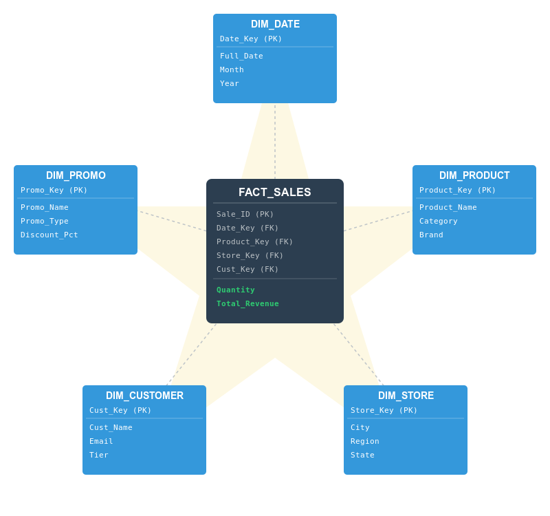
At the heart of our star is the fact table. We call this FACT_SALES, and it stores the actual business events. In this case, it records every individual sale.

Quantitative Data (Measures): The fact table contains the “numbers” that a business wants to calculate, such as revenue, quantity sold, and discount amount.
Foreign Keys (FK): It also contains a set of “Keys” (IDs) that act as pointers to the surrounding tables. These keys allow us to join the data together to see the context of each sale.

2. The Dimension Tables

Surrounding the fact table are the dimension tables. These contain the descriptive attributes (the “who, what, where, and when”) of the sale. In our example, we have five points:

DIM_DATE: Instead of just a simple timestamp, this table allows us to filter sales by year, quarter, month, or even “holiday vs. workday”.
DIM_PRODUCT: This contains details about the item sold, such as the product name, category (e.g., Electronics), brand, and unit price.
DIM_STORE: This provides geographic context. We can see which cities, regions, or specific store branches are performing best.
DIM_CUSTOMER: This holds demographic data like customer tier (Gold/Silver), name, and email, allowing us to track buying patterns.
DIM_PROMO: This helps the marketing team see the impact of specific promotions or coupons on the total revenue.

Why This Design Works

The Star Schema is the “gold standard” for data warehousing for three main reasons:

Simplicity for Users: From a user’s perspective, the logic is easy to follow. If you want to know “What was the total revenue for Electronics in New York during December?”, you simply connect the Sales table to the Product, Store, and Date tables.
Query Performance: Because the data is “denormalized” (organized into fewer tables), the database doesn’t have to perform complex calculations to find your answer. This makes reports and dashboards load much faster.
BI Tool Friendly: Almost every modern Business Intelligence tool (like Power BI, Tableau, or Looker) is specifically designed to recognize and optimize for the star schema structure.

Star schemas are denormalized by design. Those dimension tables often contain redundant information that would be split across multiple tables in a normalized database. A product dimension might store both the category name and the department name in the same row, even though category determines department.

This redundancy is intentional. It makes queries simpler and faster. Instead of joining six tables to get product information, you join to one. Business users can write queries without needing to understand complex table relationships.

The queries typically end up looking straightforward. You simply join the fact table to whatever dimensions you need, filter on dimension attributes, and aggregate the facts. Want total sales by product category and quarter? That’s just a few joins and a GROUP BY.

How Many Dimensions?

Don’t let the example above lock you into thinking star schemas need exactly five dimension tables. The number of dimensions depends entirely on your business needs and how you want to analyze the data. Our example could just as easily have looked like this:

A simple star schema might have just two or three dimensions. A sales system for a single-location business might only need a date dimension and a product dimension. An event tracking system could get by with just date and user dimensions.

On the other hand, complex analytical systems can have ten or more dimensions. A healthcare analytics warehouse might include dimensions for patients, providers, procedures, diagnoses, facilities, insurance plans, and more. As long as each dimension represents a different way to slice and analyze your facts, adding it makes sense.

The main thing to remember is that each dimension should answer a distinct question about your data: when did it happen, who was involved, what product was it, where did it occur. If you find yourself wanting to filter or group by something and it’s not in your existing dimensions, you probably need to add one.

Fact Tables: Additive vs Non-Additive

Not all measurements work the same way in fact tables. Some are additive, which means you can sum them across any dimension and get meaningful results. Sales amounts and quantities are additive.

Others are semi-additive. These can be summed across some dimensions but not others. Account balances can be summed across customers but not across time (adding yesterday’s balance to today’s balance doesn’t make sense).

Some measurements are non-additive. These can’t be summed at all. Ratios, percentages, and unit prices fall into this category. You need to calculate these from additive facts rather than storing and summing them directly.

When to Use a Star Schema

Star schemas are built for specific types of workloads and use cases. Here’s when they make sense:

Data warehousing and business intelligence. If you’re building a system specifically for reporting, dashboards, or analytics, star schemas will usually be your default choice. They’re optimized for the kinds of queries BI tools generate (aggregations across multiple dimensions with various filters).
Read-heavy workloads with infrequent updates. Star schemas work best when data is loaded in batches (daily, hourly, or in real-time streams) and then queried extensively. If you’re loading sales data once a day and then running hundreds of reports against it, that’s ideal. If you’re constantly updating individual records throughout the day, a normalized transactional database is better.
When query performance matters more than storage efficiency. The denormalization in star schemas uses more disk space than a normalized design, but makes queries significantly faster. If you have terabytes of historical data and users who expect sub-second query responses, the storage tradeoff is usually worth it.
When business users need to write their own queries. Star schemas are simple enough that analysts can understand the structure and write SQL directly, or use BI tools without needing a database expert. If your users work with tools like Tableau, Power BI, or Looker, they’ll have an easier time with a star schema than a complex normalized structure.
Historical analysis and trend tracking. Star schemas excel at time-series analysis because dimension tables typically contain slowly changing dimension (SCD) logic to track how attributes change over time. You can answer questions like “what were our sales in the Northwest region before the territory realignment” because the historical dimensional context is preserved.

You wouldn’t use a star schema for an e-commerce checkout system, a social media feed, or a real-time inventory management system. Those need the data consistency and update efficiency that normalized databases provide. Star schemas are for after the transaction happens, when you want to understand what the transactions mean.

Variations and Alternatives

The star schema isn’t the only schema you should consider. There are other options available that you may want to consider before you go ahead with your database.

The main alternative is the snowflake schema, which normalizes the dimension tables. Instead of storing category and department in the product dimension, you’d have a separate category table and a department table, with the product dimension linking to them. This saves storage space and makes dimension updates easier. For example, you can change a category name once instead of in thousands of product rows. The downside is more complex queries with additional joins, which can hurt performance. Snowflake schemas make sense when storage is expensive or when dimension tables are massive and highly redundant.

Fact constellations (or galaxy schemas) involve multiple fact tables sharing the same dimension tables. You might have separate fact tables for sales, inventory, and returns that all connect to the same product, date, and store dimensions. This is common in enterprise data warehouses where different business processes need to be analyzed both separately and together. It lets you run queries that span multiple fact tables while maintaining consistent dimensional context.

Factless fact tables are an interesting variation used to track events where there’s no measurement to record. For example, tracking student course attendance just needs to record that a student was present on a date – there’s no quantity or amount. The fact table contains only foreign keys to dimensions, but it’s still useful for counting occurrences and analyzing patterns.

Some modern approaches blur these lines entirely. Data vault modeling and data lake architectures organize data differently, prioritizing flexibility and raw data storage over query performance. These work well when requirements are unclear or constantly changing, but they typically require more processing to get query-ready data. Many organizations load raw data into a data lake, then materialize star schemas on top for actual reporting and analysis.

Getting Started

If you’re designing a star schema, start by identifying your business process and what measurements matter. Those measurements become your facts. Then figure out how users will want to slice that data. Those perspectives become your dimensions.

Keep dimension tables wide rather than deeply normalized. Make them easy to query, even if that means some redundancy. The goal is analytical simplicity, not minimizing storage space.